0. Install Package ‘SnapMatch’

You need to install package optmatch, rcbalance before installing the [SnapMatch] package. It is recommanded to install package lpSolve and RItools as well.

install.packages('optmatch')
install.packages('rcbalance')
install.packages('lpSolve')
install.packages('RItools')
library('optmatch')
library('rcbalance')
library('lpSolve')
library('RItools')
library('SnapMatch')

1. Snapshot Matching

1.1 Optimal Snapshot Matching

1.2 Nearest (Greedy) Snapshot Matching

Put some introduction here.

2. Optimal Snapshot Matching Example

2.1 Load Demo Data

The demo dataset contains 20 subjects in the treatment group and 100 subject in the control group. Each subject in the control group has 5 time points.

dat <- SnapMatch:::demo()
head(dat)

##   id trt         X1 X2
## 1 t1   1 -1.5604756  0
## 2 t2   1 -1.2301775  1
## 3 t3   1  0.5587083  1
## 4 t4   1 -0.9294916  1
## 5 t5   1 -0.8707123  0
## 6 t6   1  0.7150650  0

tail(dat)

##       id trt         X1 X2
## 515  c99   0  1.1146485  2
## 516 c100   0  0.5500440  1
## 517 c100   0  1.2366758  3
## 518 c100   0  0.1390979  1
## 519 c100   0  0.4102751  2
## 520 c100   0 -0.5584569  5

2.2 Match With Covariate Distance

We can match by mahalanobis/euclidean/rank_mahalanobis distance.

  # calculate the distance matrix
dis <- match_on(trt~X1+X2, data = dat, method="mahalanobis")
  # conduct optimal matching. 'Id' is the id column for each subject
pm <- optmatch_snap(dis, data = dat, id = 'id')
  # plot result
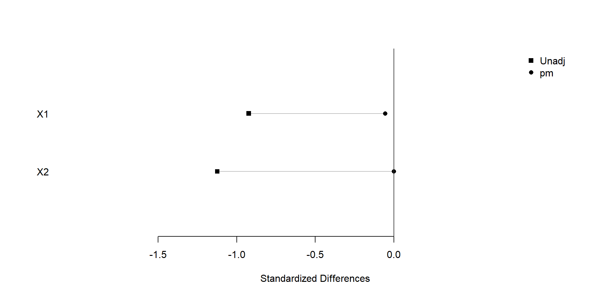
plot(xBalance(trt ~ X1+X2+strata(pm), data=dat), xlim=c(-2,1), ylim=c(0,3))

We find that covariate balance is achieved after snapshot matching.

2.3 Match With Propensity Score

  # calculate propensity score
prop <- glm(trt ~ X1+X2, data = dat, family = binomial())
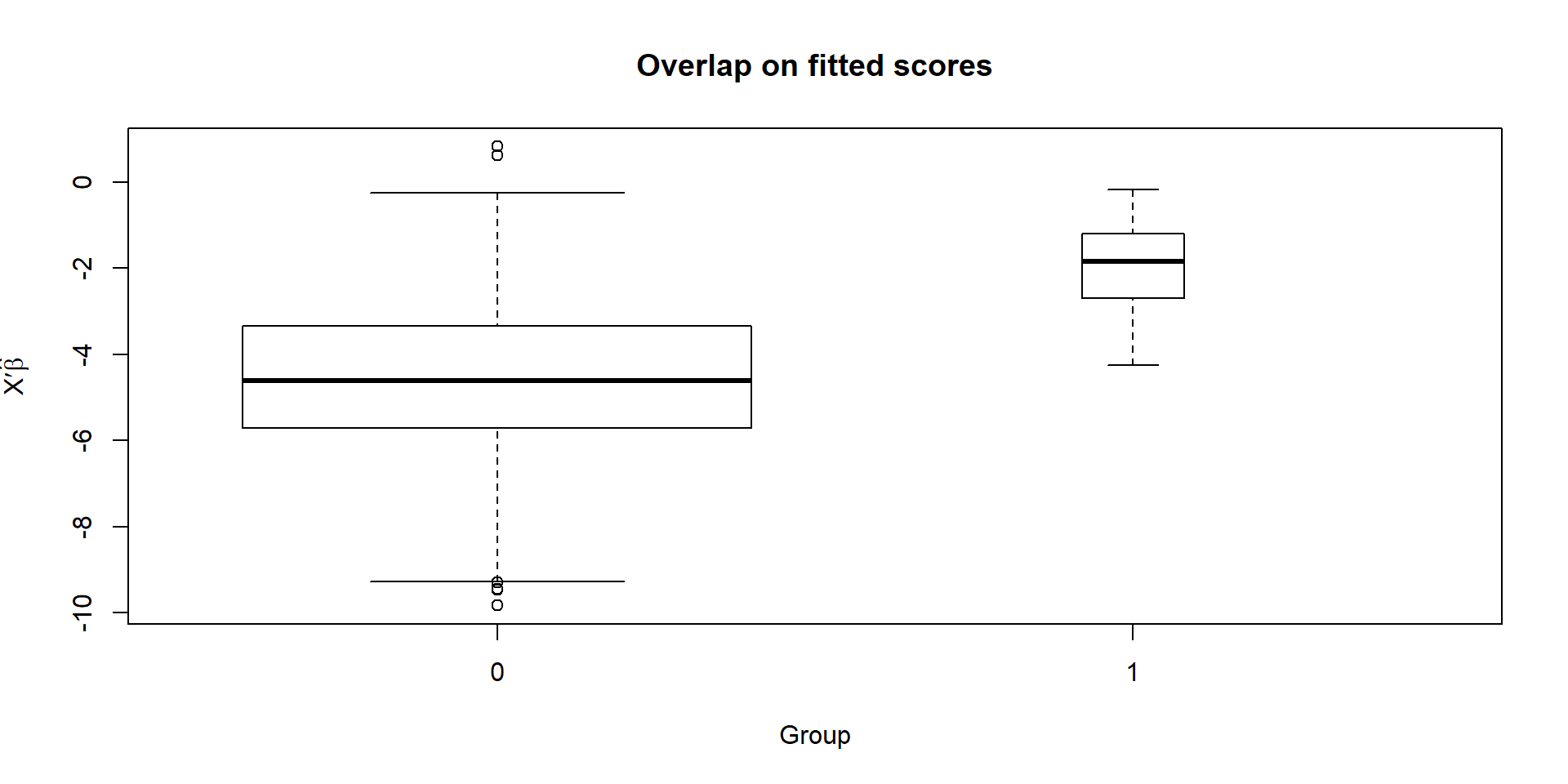
boxplot(prop)

The groups do overlap, if not greatly. It may be wise to restrict the sample to the region of overlap, at least roughly.

  # conduct optimal matching by propensity score. 'Id' is the id column for each subject
pm <- optmatch_snap(trt ~ X1+X2, data = dat, id = 'id')
  # plot result
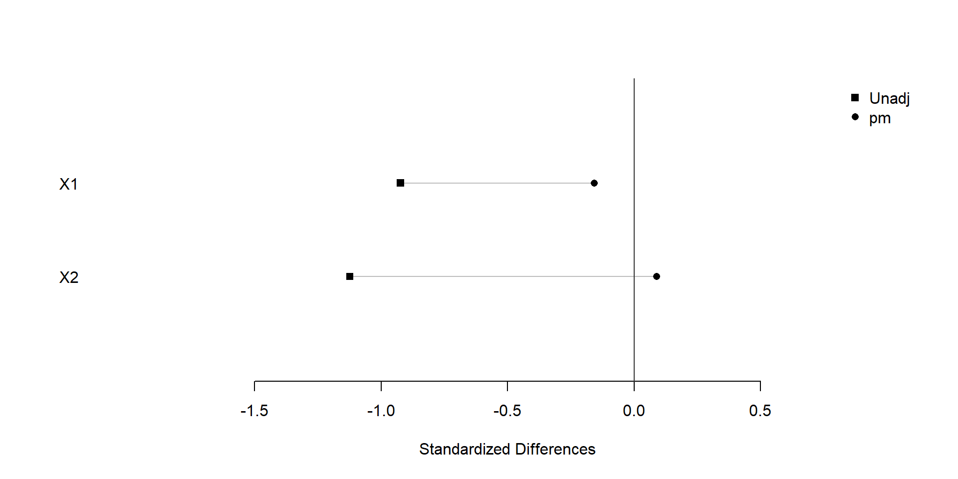
plot(xBalance(trt ~ X1+X2+strata(pm), data=dat), xlim=c(-2,1), ylim=c(0,3))

We find that similar covariate balance is achieved after snapshot matching.

2.4 Complex Match With ‘match_on’ Function

The package accepts ‘match_on’ function from ‘optmatch’ package as a distance matrix. For example, here we show how to perform a snapshot matching within a propensity score caliper.

  # calculate distance by propensity score
dis <- match_on(glm(trt ~ X1+X2, data = dat, family = binomial()))
dis[1:5,1:5]

##          control
## treatment       21        22        23        24        25
##         1 3.438599 1.5015123 2.2027200 2.9487052 1.4033947
##         2 2.488007 0.5509201 1.2521277 1.9981130 0.4528025
##         3 1.434081 0.5030065 0.1982011 0.9441864 0.6011241
##         4 2.310857 0.3737702 1.0749779 1.8209631 0.2756526
##         5 3.032224 1.0951365 1.7963441 2.5423294 0.9970189

  # add caliper
dis <- caliper(dis,2) + dis
dis[1:5,1:5]

##        control
## treated       21        22        23        24        25
##       1      Inf 1.5015123       Inf       Inf 1.4033947
##       2      Inf 0.5509201 1.2521277 1.9981130 0.4528025
##       3 1.434081 0.5030065 0.1982011 0.9441864 0.6011241
##       4      Inf 0.3737702 1.0749779 1.8209631 0.2756526
##       5      Inf 1.0951365 1.7963441       Inf 0.9970189

  # conduct optimal snapshot matching
pm <- optmatch_snap(dis, data = dat, id = 'id')
  # plot result
plot(xBalance(trt ~ X1+X2+strata(pm), data=dat), xlim=c(-2,1), ylim=c(0,3))

3. Nearest Snapshot Matching Example

3.1 Load Demo Data