Zero Inflated Poisson Factor Analysis (R Verison)
0. Install Package ‘ZIPFA’
You need to install package optimx, trustOptim before installing ZIPFA.
install.packages('optimx')
install.packages('trustOptim')
install.packages('ZIPFA')
library('Matrix')
library('parallel')
library('doParallel')
library('foreach')
library('optimx')
library('trustOptim')
library('ZIPFA')
1. Zero Inflated Poisson Regression
Let’s introduce the zero inflated Poisson regression where the logit true zero probability is negatively associated with log Poisson expectation.
Let the response variable be \(Y=(y_1,y_2,\ldots,y_n)^\top\) following a zero-inflated Poisson distribution:
\[ Y_i\sim \begin{cases} 0, & \text{with prob} = p_i\\ Poisson(m_i \lambda_i), & \text{with prob} = 1-p_i \end{cases} \] where \(m=(m_1,m_2,\cdots,m_n)^\top\) is the known scaling vector and takes the value of constant 1 in most cases. Let \(X\) be an \(n\) by \(p\) design matrix, where column vector \(X_i\) denotes the i row of \(X\); \(\beta =(b_1, b_2,\ldots, b_{p})^\top\) is the coefficient vector to be estimated.
With the aforementioned relationship between \(p_i\) and \(\lambda_i\), the model satisfies: \[
\ln \operatorname{E}(Y_i/m_i|X_i)=\ln(\lambda_i)=X_i^\top\beta \qquad \text{and}\qquad \text{logit}(p_i)=-\tau\ln(\lambda_i).
\]
1.1 Simulation Data
  # sample size
n <- 5000
  # variable x1
x1 <- rnorm(n)
  # variable x2
x2 <- rnorm(n)
  # beta_0 = 1.5, beta_1 = 1, beta_2 = -2
lam <- exp(x1 - 2*x2 + 1.5)
  # generate the Poisson part, m = 1
y <- rpois(n, lam)
  # tau = 0.75
tau <- 0.75
  # true zero prabability p
p <- 1./(1+lam^tau)
Z <- rbinom(n, 1, p)
  # replace some values with true zeros
y[as.logical(Z)] <- 0
1.2 Model Estimation
We use function EMzeropoisson_mat() to build the zero inflated Poisson regression.
  # run the regression
res <- EMzeropoisson_mat(matrix(c(y,x1,x2),ncol=3), Madj = FALSE, intercept = TRUE)
## Initialzing...## Start maximizing...## This is 2 th iteration, Frobenius norm diff = 0.186327.## This is 3 th iteration, Frobenius norm diff = 0.0476255.## This is 4 th iteration, Frobenius norm diff = 0.00976385.## This is 5 th iteration, Frobenius norm diff = 0.00185416.## This is 6 th iteration, Frobenius norm diff = 0.000346737.## This is 7 th iteration, Frobenius norm diff = 6.46548e-05. # get fitted tau
fittedtau <- res[nrow(res),1]
fittedtau## [1] 0.7653681 # get fitted intercept
fittedintercept <- res[nrow(res),2]
fittedintercept## [1] 1.50815 # get fitted beta
fittedbeta <- res[nrow(res),-(1:2)]
fittedbeta## [1] 0.9997759 -1.9974022We get the estimated intercept 1.508, \(\beta_1 =\) 0.9998, \(\beta_2 =\) -1.997, \(\tau =\) 0.7654, which are the parameters we used to generate the data.
Usage of EMzeropoisson_mat():
fittedbeta <- EMzeropoisson_mat(data, tau = 0.1, initial = NULL, initialtau = ‘iteration’, tol = 1e-4, maxiter = 100, Madj = FALSE, m = NULL, display = TRUE, intercept = TRUE)
– data: A matrix with the first columns is y and the rest columns are x.
– tau (0.1): Initial tau value to fit. Will be overwritten by the first value in initial argument.
– ‘initial’ (NULL): A list of initial values for the fitting. c(tau beta).
– ‘initialtau’ (‘iteration’): A character specifying the way to choose the initial value of tau at the beginning of EM iteration.
‘stable’: estimate tau from fitted beta in last round;
‘initial’: always use the initially assigned tau in ‘tau’ or ‘initial’;
Use the default tau = 0.1 if ‘initial’ is empty.
‘iteration’: use fitted tau in last round.
– ‘tol’ (1e-4): Percentage of l2 norm change of [tau beta].
– ‘maxiter’ (100): Max iteration number.
– ‘Madj’ (FALSE): If TRUE then adjust for relative library size M.
– ‘m’ (NULL): A vector containing relative library size M.
– ‘display’ (TRUE): If TRUE display the fitting procedure.
– ‘intercept’ (TRUE): If TRUE then the model contains an intercept.
The function turns a matrix. Each row is fitted value in each iteration. The last row the final result. The first column is fitted \(\tau\). If intercept is TRUE, then the second column is the intercept, and the rest columns are other coefficients. If intercept is FALSE, the rest columns are other coefficients.
2. Zero Inflated Poisson Factor Analysis
In microbiome studies, the absolute sequencing read counts are summarized in a matrix \(A \in \mathbb{N}_0^{n\times m}\), where \(n\) is the sample size and \(m\) is the number of taxa. Let \(A_{ij}\) represents the read count of taxon \(j\) of individual \(i\) \((i=1,\cdots,n;\, j=1,\cdots,m)\). Let \(N = (N_1,N_2,\cdots,N_n)^\top\) a be vector of the relative library sizes where: \[ N_i =\sum_{j=1}^m A_{ij}\bigg/\operatorname{median}\left( \sum_{j=1}^m A_{1j},\; \sum_{j=1}^m A_{2j},\; \cdots,\; \sum_{j=1}^m A_{nj} \right). \] Since excessive zeros may come from true absence or undetected presence of taxa, a mixed distribution is proper to describe \(A_{ij}\). It is reasonable to assume each read count \(A_{ij}\) follows a zero-inflated Poisson (ZIP) distribution: \[ A_{ij}\sim \begin{cases} 0, & \text{with prob }= p_{ij}\\ Poisson(N_i\lambda_{ij}), & \text{with prob }= 1-p_{ij} \end{cases} \] where \(p_{ij}\; (0\le p_{ij} \le 1)\) is the unknown parameter of the Bernoulli distribution that describes the occurrence of true zeros; \(\lambda_{ij}\; (\lambda>0)\) is the unknown parameter of the normalized Poisson part, and \(N_i \lambda_{ij}\) is the Poisson rate adjusted by the subject-specific relative library size \(N_{i}\). Then let \(P = \operatorname{logit}(p_{ij}) \in \mathbb{R}^{n\times m}\) and \(\Lambda = \ln( \lambda_{ij})\in \mathbb{R}^{n\times m}\) be the corresponding natural parameter matrices to map parameters \(p_{ij}\), \(\lambda_{ij}\) to the real line.
To link the negative relationship between true zero probability \(p_{ij}\) and Poisson rate \(\lambda_{ij}\), we propose to use a positive shape parameter \(\tau\) to build the logistic link by modeling \(P=-\tau \Lambda\) (i.e., \(\operatorname{logit}(p_{ij})=-\tau \ln(\lambda_{ij})\)).
To encourage dimension reduction, we assume matrix \(\Lambda \in \mathbb{R}^{n\times m}\) has a low rank structure \(\Lambda = UV^\top\) with rank \(K<\min(m, n)\), where \(U\in \mathbb{R}^{n\times K}\) is the score matrix; \(V \in \mathbb{R}^{m\times K}\) is the loading matrix. Then the proposed ZIPFA model with rank \(K\) is given by: \[ \begin{cases} A_{ij}\sim \text{ZIP distribution}\\ \operatorname{logit}(p_{ij})=-\tau \ln(\lambda_{ij}) \\ %\quad \left(p_{ij}=\frac{1}{1+\lambda_{ij}^\tau}\right)\\ \ln (\lambda_{ij})=u_{i1}v_{j1}+u_{i2}v_{j2}+\cdots+u_{iK}v_{jK} \end{cases} \] where \(u_{ij}\), \(v_{ij}\) are elements of \(U\), \(V\). Here, \(u_{ij}\) represents the j factor score for the i individual, and \(v_{ij}\) is the i taxon loading on j factor.
2.1 Simulation Data
We generate rank-3 synthetic NGS data of \(200\) samples (\(n=200\)) and \(100\) taxa (\(m=100\)) according to the model assumption. The Poisson logarithmic rate matrix \(\Lambda=UV^\top\), where \(U\in \mathbb{R}^{m\times 3}\) is a left singular vector matrix, and \(V\in \mathbb{R}^{n\times 3}\) is a right singular vector matrix. We consider three different clustering patterns in the samples as depicted in \(U\). To generate \(U\), we create a 200-by-3 matrix \(U\) such that: \[\begin{alignat*}{2} &U(36:80,1)=2.0,&\qquad &U(81:140,1)=1.7\\ &U(1:35,2)=1.8,&\qquad &U(36:80,2)=0.9\\ &U(36:200,3)=1.7&& \end{alignat*}\] with all the other entries being 0, and then jitter all the entries by adding random numbers generated from \(N(0, 0.06^2\)). Similarly, To generate \(V\), we create a 100-by-3 matrix \(V\) such that: \[\begin{alignat*}{2} &V(61:100,1)=1.7& &\\ &V(36:60,2)=1.7,&\qquad &V(61:100,2)=1.0\\ &V(1:25,3)=1.7,&\qquad& V(26:100,3)=0.9 \end{alignat*}\] with all the other entries being 0, and then jitter all the entries by adding random numbers generated from \(N(0, 0.05^2)\). The three columns of \(U\) and \(V\) are plotted in the columns of Figure 1(a) and the true \(\ln(\lambda)\) matrix is plotted in Figure 1(b). Each row in \(U\) corresponds to one sample and each row in \(V\) indicates one taxon profile. In Figure 1(c),(d), we applied complete linkage hierarchical clustering to \(U\), \(V\). It is clear that both taxa and samples could be clustered into \(4\) groups.
We generate matrix \(A^\circ\) that \(A_{ij}^\circ \sim Poisson(N_i\lambda_{ij})\) where the scaling parameter \(N_i\) is set to be \(1\). Also we need true zero probability \(p_{ij}\) to generate inflated zeros:
\[ \operatorname{logit}(p_{ij})=-\tau \ln(\lambda_{ij}) \quad (p_{ij}=\frac{1}{1+\lambda_{ij}^\tau}) \]
We adjust the total percentage of excessive zeros by setting different \(\tau\) values. Once \(p_{ij}\) is generated, our simulated NGS data matrix \(A\) can be obtained by replacing \(A^\circ_{ij}\) with \(0\) with the probability of \(p_{ij}\).
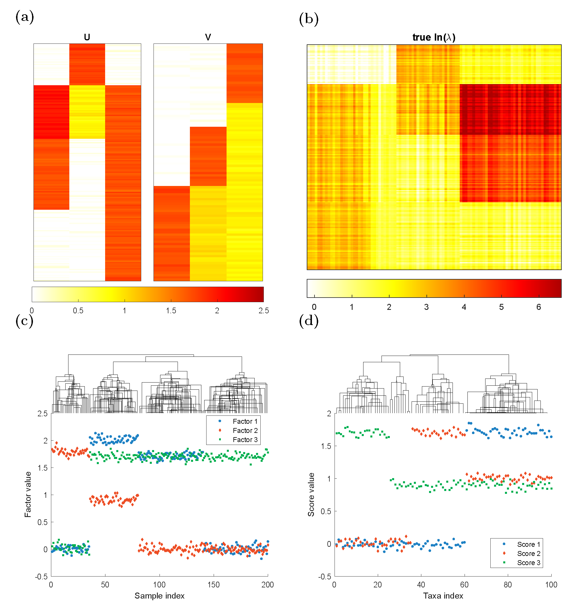
Figure 1. Plots of simulation parameters. (a) True left singular vectors \(U\) and true right singular vector \(V\), indicating taxon clusters. (b) Heatmap of true \(\ln(\lambda)\) matrix. (c)(d) The factor values for each sample/taxa. They could be clustered into 4 groups.
set.seed(1)
  # Matrix U, V
u <- c(rep(0,35), rep(2,45), rep(1.7, 60), rep(0,60), rep(1.8,35), rep(0.9,45), rep(0,120), rep(0,35), rep(1.7,165))
u <- matrix(u, byrow = F, ncol = 3)
vt <- c(rep(0,30), rep(0,30), rep(1.7,40), rep(0,35), rep(1.7,25), rep(1,40), rep(1.7,25), rep(0.9,50), rep(0.9,25))
vt <- matrix(vt, byrow = T, nrow = 3)
u <- rnorm(600,0,0.06)+u
vt <- rnorm(300,0,0.05)+vt
  # Lambda matrix
a <- u %*% vt
  # lambda_{ij}
lambda <- exp(a)
  # Poisson Part
X <- rpois(20000, lambda)
X <- matrix(X, byrow = F, nrow = 200)
  # tau value
tau <- 0.616
  # add true zeros
P <- 1./(1+lambda^tau)
Z <- rbinom(20000,size = 1,P)
X[as.logical(Z)] <- 0
2.2 Model Estimation with Specified Rank
We use function ZIPFA() to conduct the zero inflated Poisson factor analysis.
  # run the model (rank = 3)
res <- ZIPFA(X, k = 3, Madj = F, display = F)

  # fitted U, V
fittedU <- res$Ufit[[res$itr]]
fittedV <- res$Vfit[[res$itr]]

  # iteration number, fitted tau, likelihood in each iteration
itr <- res$itr
itr
## [1] 4fittedtau <- res$tau
fittedtau##
## 0.6056028likelihood <- res$Likelihood
likelihood## [1] -56705.30 -53082.90 -52994.18 -52982.86The algorithm converges in 4 iterations with fitted \(\tau =\) 0.6056. The likelihood increases during the fitting procedure. The heatmap of \(U V^\top\) is in Figure 2.
Usage of ZIPFA():
res <- ZIPFA(X, k, tau = 0.1, cut = 0.8, tolLnlikelihood = 5e-4, iter = 20, tol = 1e-4, maxiter = 100, initialtau = ‘iteration’, Madj = TRUE, display = TRUE, missing = NULL)
– X: The matrix to be decomposed.
– k: The number of factors.
– tau (0.1): Initial tau value to fit. Will be overwritten by the first value in initial argument.
– ‘cut’ (0.8): To delete columns that has more than 100(‘Cut’)% zeros. Cut = 1, if no filtering.
– ‘tolLnlikelihood’ (5e-4): The max percentage of log likelihood differences in two iterations.
– ‘iter’ (20): Max iteration number in the zero inflated poisson regression.
– ‘tol’ (1e-4): Percentage of l2 norm change of [tau beta] in ZIP regression.
– ‘maxiter’ (100): Max iterations in ZIP regression.
– ‘initialtau’ (‘iteration’): A character specifying the way to choose the initial value of tau at the beginning of EM iteration.
‘stable’: estimate tau from fitted beta in last round;
‘initial’: always use the initially assigned tau in ‘tau’ or ‘initial’;
Use the default tau = 0.1 if ‘initial’ is empty.
‘iteration’: use fitted tau in last round.
– ‘Madj’ (TRUE): If TRUE then adjust for relative library size M.
– ‘display’ (TRUE): If TRUE display the fitting procedure.
– ‘missing’ (NULL): T/F matrix. If ‘missing’ is not empty, then CVLikelihood is likelihood of X with missing = T.
Result contains the fitted U (a list containing fitted U matrix in each iteration and the last one is the final fit), V (a list containing fitted U matrix in each iteration and the last one is the final fit), iteration number, model total likelihood.
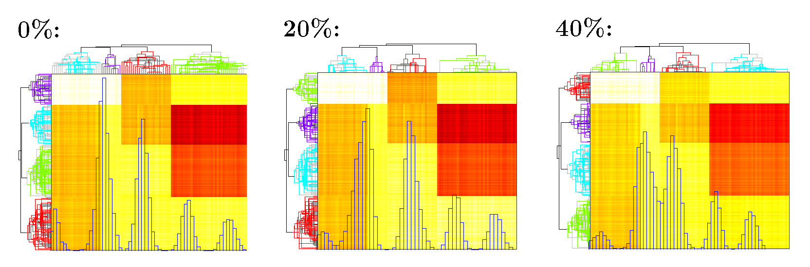
Figure 2. Heatmap of \(\widehat U\widehat V^\top\) under different percentage of inflated zeros. Blue histogram shows the distribution of fitted \(\widehat U\widehat V^\top\); Phylogenetic tree on the top and left shows clustering of taxa and samples.
2.3 Cross Validation to Choose Rank
We use function cv_ZIPFA() to conduct the zero inflated Poisson factor analysis. (The R version is slow. Use the Matlab version if possible. Or reduce the number of folds.)
  # do cross validation without parallel computing (rank = 2 to 6)
CVlikelihood <- cv_ZIPFA(X, fold = 10, k = 2:6, Madj = F, parallel = F)

apply(CVlikelihood,2,median)

   -6796   -5380   -5400   -5426   -5462
The function returns a matrix. Each row in ‘CVlikelihood’ represents the CV likelihood of one fold and each column is for specified rank (from 2 to 6). The median CV likelihood reaches its maximum value when rank equals to 3 in Figure 3, which is the rank we used to generate the simulation data.
Usage of cv_ZIPFA():
CVlikelihood <- cv_ZIPFA(X, k, fold, tau = 0.1, cut = 0.8, tolLnlikelihood = 5e-4, iter = 20, tol = 1e-4, maxiter = 100, initialtau = ‘iteration’, Madj = TRUE, display = TRUE, parallel = FALSE)
– X: The matrix to be decomposed.
– k: A vector containing the number of factors to try.
– fold (10): The number of folds used in cross validation.
– tau (0.1): Initial tau value to fit. Will be overwritten by the first value in initial argument.
– ‘cut’ (0.8): To delete columns that has more than 100(‘Cut’)% zeros. Cut = 1, if no filtering.
– ‘tolLnlikelihood’ (5e-4): The max percentage of log likelihood differences in two iterations.
– ‘iter’ (20): Max iteration number in the zero inflated poisson regression.
– ‘tol’ (1e-4): Percentage of l2 norm change of [tau beta] in ZIP regression.
– ‘maxiter’ (100): Max iterations in ZIP regression.
– ‘initialtau’ (iteration’): A character specifying the way to choose the initial value of tau at the beginning of EM iteration.
‘stable’: estimate tau from fitted beta in last round;
‘initial’: always use the initially assigned tau in ‘tau’ or ‘initial’;
Use the default tau = 0.1 if ‘initial’ is empty.
‘iteration’: use fitted tau in last round.
– ‘Madj’ (TRUE): If TRUE then adjust for relative library size M.
– ‘display’ (TRUE): If TRUE display the fitting procedure. Info in ZIPFA will not be shown in ‘Parallel’ mode even ‘Display’ is TRUE
– ‘parallel’ (FALSE): Use doParallel and foreach package to accelerate.
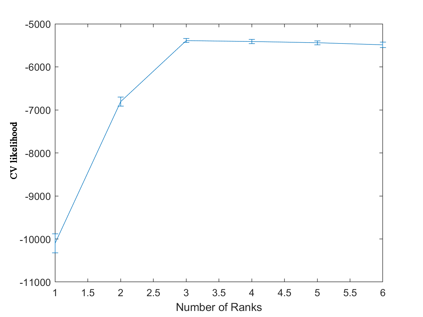
Figure 3. CV likelihood vs. number of ranks